Non-Reversible Parallel Tempering#
In Notebook 04 we saw that single-chain Gibbs sampling fails for multimodal distributions — the chain gets stuck in one energy basin. Parallel tempering (PT) solves this by running multiple chains at different temperatures and swapping states between them.
This notebook covers: - The parallel tempering idea and why it works - Deterministic Even-Odd (DEO) swaps — non-reversible is better - Round trip diagnostics: Λ, τ, efficiency - Adaptive schedule optimization — concentrate chains where they matter - Automatic chain count discovery - Head-to-head: naive vs optimized vs more chains - Full pipeline: discover → adapt → sample
The algorithms are based on Syed et al. (2021), "Non-Reversible Parallel Tempering: a Scalable Highly Parallel MCMC Scheme" (arXiv:1905.02939).
import jax
import jax.numpy as jnp
import matplotlib.pyplot as plt
import numpy as np
import time

from hamon import SpinNode, Block, NRPTStateObserver

from hamon.models.ising import IsingEBM, IsingSamplingProgram, hinton_init
from hamon.nrpt import nrpt
from hamon.tuning import tune_schedule, tune_chains
Helper: build an L×L Ising grid#
We'll reuse this throughout the notebook. Checkerboard coloring gives us two blocks for parallel Gibbs updates.
def make_ising_grid(L, coupling=1.0, field=0.0):
    """LxL nearest-neighbor Ising model with checkerboard blocking."""
    nodes_2d = [[SpinNode() for _ in range(L)] for _ in range(L)]
    nodes = [n for row in nodes_2d for n in row]
    edges = []
    for i in range(L):
        for j in range(L):
            if j + 1 < L:
                edges.append((nodes_2d[i][j], nodes_2d[i][j + 1]))
            if i + 1 < L:
                edges.append((nodes_2d[i][j], nodes_2d[i + 1][j]))
    biases = jnp.ones(len(nodes)) * field
    weights = jnp.ones(len(edges)) * coupling
    even = [nodes_2d[i][j] for i in range(L) for j in range(L) if (i + j) % 2 == 0]
    odd = [nodes_2d[i][j] for i in range(L) for j in range(L) if (i + j) % 2 == 1]
    free_blocks = [Block(even), Block(odd)]
    return nodes, nodes_2d, edges, biases, weights, free_blocks
The multimodality problem#
At low temperature, the ferromagnetic Ising model has two deep energy minima (all +1 and all -1). A single Gibbs chain can't cross the barrier between them.
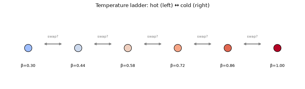
The parallel tempering idea: - Run \(N\) chains at different inverse temperatures \(\beta_0 < \beta_1 < \ldots < \beta_{N-1}\) - The hot chain (\(\beta_0 \approx 0\)) explores freely — it can cross barriers - The cold chain (\(\beta_{N-1}\) = target) samples from the distribution we care about - Swap states between adjacent chains — hot-chain exploration propagates down to cold
# Schematic: temperature ladder
fig, ax = plt.subplots(figsize=(10, 3))
n_demo = 6
betas_demo = np.linspace(0.3, 1.0, n_demo)

for i, b in enumerate(betas_demo):
    color = plt.cm.coolwarm(b / 1.0)
    ax.scatter(i, 0, s=300, color=color, zorder=5, edgecolors="black")
    ax.text(i, -0.15, f"\u03b2={b:.2f}", ha="center", fontsize=9)
    if i < n_demo - 1:
        ax.annotate(
            "",
            xy=(i + 0.7, 0.03),
            xytext=(i + 0.3, 0.03),
            arrowprops=dict(arrowstyle="<->", color="gray", lw=2),
        )
        ax.text(i + 0.5, 0.08, "swap?", ha="center", fontsize=8, color="gray")

ax.set_xlim(-0.5, n_demo - 0.5)
ax.set_ylim(-0.3, 0.3)
ax.set_title("Temperature ladder: hot (left) \u2194 cold (right)")
ax.axis("off")
plt.tight_layout()
plt.show()
Setup: 16×16 ferromagnetic Ising model#
We use a 16×16 ferromagnet with target \(\beta = 1.0\) (past the critical point \(\beta_c \approx 0.44\)). At this temperature the system is in the ordered phase with two degenerate ground states separated by a free-energy barrier at the phase transition.
L = 16
nodes, nodes_2d, edges, biases, weights, free_blocks = make_ising_grid(L, coupling=1.0)

print(f"Ferromagnet: {L}x{L} = {L * L} spins, {len(edges)} edges (all J=+1)")
print("Target \u03b2 = 1.0  (\u03b2_c ~ 0.44)")
The easy way: autosample#
Choosing the number of chains, the number of local Gibbs sweeps between
swaps, and the temperature schedule can all be done in one call with
autosample. It autotunes all three (the exploration count is calibrated to
your hardware) and draws from the cold chain. The rest of this notebook
unpacks what it does under the hood.
This cell uses autotune's defaults (n_tune=4, rounds_per_probe=400, n_rounds=1000); the manual pipeline at the end of the notebook is set to the same budgets, so the reported round-trip efficiency is directly comparable. The only deliberate difference is gibbs_steps_per_round: autotune calibrates it to the device (~2 on CPU), the manual run fixes 4.
from hamon import autosample

N_ROUNDS = 1000
GIBBS_STEPS = 4

ebm = IsingEBM(nodes, edges, biases, weights, jnp.array(1.0))
program = IsingSamplingProgram(ebm, free_blocks, [])


def init_factory(n_chains, ebms, programs):
    fb = programs[0].gibbs_spec.free_blocks
    ks = jax.random.split(jax.random.key(7), n_chains)
    return [hinton_init(ks[c], ebms[0], fb, ()) for c in range(n_chains)]


# Uses autotune's defaults (n_tune=4, rounds_per_probe=400, n_rounds=1000); the
# manual pipeline at the end of the notebook is set to the same budgets, so the
# reported round-trip efficiency is directly comparable. n_expl is autotuned --
# on this CPU it picks ~2 (best ESS/compute), where the manual run fixes 4.
samples, report = autosample(
    jax.random.key(0),
    n_samples=1000,
    ebm=ebm,
    program=program,
    init_factory=init_factory,
    clamp_state=[],
    beta_range=(0.3, 1.0),
    sample_nodes=nodes,
    max_exploration_steps=5,
)
print(report.summary())
print("samples:", samples.shape)
NRPT health: round-trip efficiency 0.192 despite an equalized schedule (rejection std=0.053): the local exploration kernel limits mixing (ELE violation). Raise gibbs_steps_per_round, or increase N to ~17.
AUTOTUNE: N=19  n_expl=1  Lambda=6.610  device=None
  exploration: chose n_expl=1 (ESS/sec=543.1, t_round=0.122 ms)
  round trips: 16 over 1000 rounds  tau_obs=0.0160  tau_pred=0.0650  efficiency=0.246
samples: (1000, 256)
Basic NRPT with nrpt#
The nrpt function runs non-reversible parallel tempering. We need:
- A list of EBMs (one per chain, at different \(\beta\) values)
- A list of sampling programs
- Initial states for each chain
hamon exploits temperature linearity of the Ising energy: \(E_\beta = \beta \cdot E_{\text{base}}\). This means swap decisions need only one energy evaluation per chain instead of four per pair.
n_chains = 8
betas = jnp.linspace(0.3, 1.0, n_chains)

ebms = [IsingEBM(nodes, edges, biases, weights, jnp.array(float(b))) for b in betas]
programs = [IsingSamplingProgram(e, free_blocks, []) for e in ebms]

key = jax.random.key(42)
keys = jax.random.split(key, n_chains + 1)
init_states = [hinton_init(keys[i], ebms[0], free_blocks, ()) for i in range(n_chains)]

states, stats = nrpt(
    keys[-1],
    ebms,
    programs,
    init_states,
    clamp_state=[],
    n_rounds=500,
    gibbs_steps_per_round=GIBBS_STEPS,
)

print(f"Chains: {n_chains}")
print(f"Betas:  {[f'{b:.3f}' for b in betas]}")
print(f"Rejection rates:  {[f'{float(r):.3f}' for r in stats['rejection_rates']]}")
Chains: 8
Betas:  ['0.300', '0.400', '0.500', '0.600', '0.700', '0.800', '0.900', '1.000']
Rejection rates:  ['0.976', '0.988', '0.936', '0.712', '0.572', '0.352', '0.200']
DEO swaps explained#
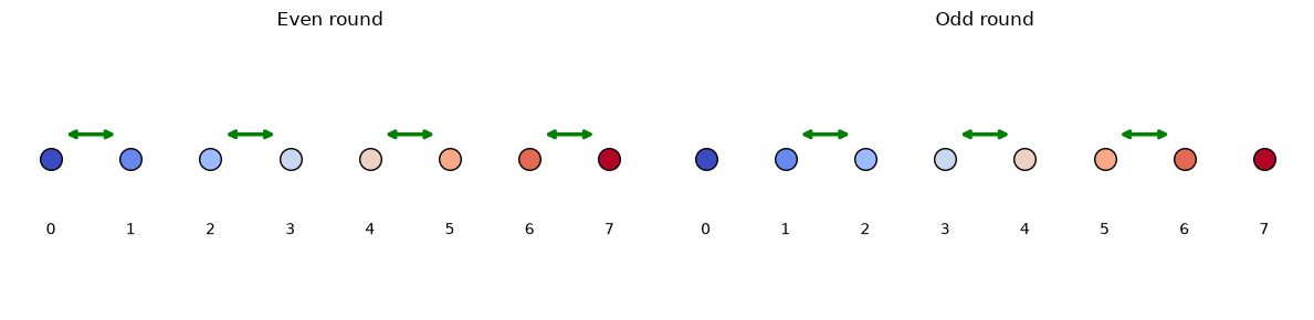
hamon uses Deterministic Even-Odd (DEO) swaps, which are key to non-reversibility:
- Even rounds: attempt swaps between pairs (0,1), (2,3), (4,5), ...
- Odd rounds: attempt swaps between pairs (1,2), (3,4), (5,6), ...
- The parity alternates deterministically: even, odd, even, odd, ...
This is non-reversible because the sequence even→odd→even is not the same forwards and backwards. Syed et al. (2021) proved this gives strictly better round trip rates than random swaps.
# Visualize the DEO swap pattern
fig, axes = plt.subplots(1, 2, figsize=(12, 3))

for ax, parity, title in zip(axes, ["even", "odd"], ["Even round", "Odd round"]):
    for i in range(n_chains):
        ax.scatter(
            i,
            0,
            s=200,
            color=plt.cm.coolwarm(i / (n_chains - 1)),
            edgecolors="black",
            zorder=5,
        )
        ax.text(i, -0.15, f"{i}", ha="center", fontsize=10)

    if parity == "even":
        swap_pairs = [(i, i + 1) for i in range(0, n_chains - 1, 2)]
    else:
        swap_pairs = [(i, i + 1) for i in range(1, n_chains - 1, 2)]

    for a, b in swap_pairs:
        ax.annotate(
            "",
            xy=(b - 0.15, 0.05),
            xytext=(a + 0.15, 0.05),
            arrowprops=dict(arrowstyle="<->", color="green", lw=2.5),
        )

    ax.set_xlim(-0.5, n_chains - 0.5)
    ax.set_ylim(-0.3, 0.25)
    ax.set_title(title)
    ax.axis("off")

plt.tight_layout()
plt.show()
Round trip diagnostics#
The quality of parallel tempering is measured by how efficiently information flows from hot to cold chains:
- \(\Lambda\) (global communication barrier): sum of local barriers. Higher \(\Lambda\) = harder problem.
- \(\tau_{\text{predicted}}\): theoretical optimal round trip rate = \(1/(2 + 2\Lambda)\)
- \(\tau_{\text{observed}}\): actual round trip rate from tracking the index process
- Efficiency: \(\tau_{\text{observed}} / \tau_{\text{predicted}}\) — how close to optimal
diag = stats["round_trip_diagnostics"]

print("Round trip diagnostics")
print(f"  Global barrier \u039b:       {float(diag['Lambda']):.4f}")
print(f"  Predicted \u03c4 = 1/(2+2\u039b): {float(diag['tau_predicted']):.4f}")
print(f"  Observed \u03c4:             {float(diag['tau_observed']):.4f}")
print(f"  Efficiency (\u03c4_obs/\u03c4):   {float(diag['efficiency']):.4f}")
print()
print(f"  Round trips per machine: {diag['round_trips_per_chain'].tolist()}")
print(f"  Restarts per machine:    {diag['restarts_per_chain'].tolist()}")
Round trip diagnostics
  Global barrier Λ:       4.7360
  Predicted τ = 1/(2+2Λ): 0.0872
  Observed τ:             0.0060
  Efficiency (τ_obs/τ):   0.0688

  Round trips per machine: [0, 0, 0, 1, 1, 0, 0, 1]
  Restarts per machine:    [1, 0, 1, 2, 1, 1, 1, 2]
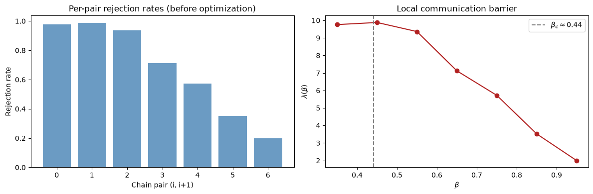
Communication barrier \(\lambda(\beta)\)#
The local communication barrier \(\lambda(\beta)\) measures how hard it is to swap at each temperature. Peaks in \(\lambda(\beta)\) indicate where the schedule needs more chains. For the 2D Ising model, this peaks near the critical temperature \(\beta_c \approx 0.44\).
lambda_profile = diag["lambda_profile"]
beta_midpoints = (betas[:-1] + betas[1:]) / 2

fig, axes = plt.subplots(1, 2, figsize=(12, 4))

axes[0].bar(
    range(len(stats["rejection_rates"])),
    np.array(stats["rejection_rates"]),
    color="steelblue",
    alpha=0.8,
)
axes[0].set_xlabel("Chain pair (i, i+1)")
axes[0].set_ylabel("Rejection rate")
axes[0].set_title("Per-pair rejection rates (before optimization)")

axes[1].plot(
    np.array(beta_midpoints), np.array(lambda_profile), "o-", color="firebrick"
)
axes[1].axvline(0.4407, color="gray", ls="--", label="$\\beta_c \\approx 0.44$")
axes[1].set_xlabel("$\\beta$")
axes[1].set_ylabel("$\\lambda(\\beta)$")
axes[1].set_title("Local communication barrier")
axes[1].legend()

plt.tight_layout()
plt.show()
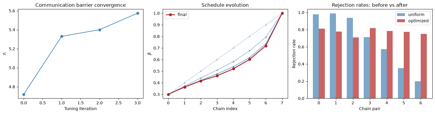
Adaptive schedule optimization with tune_schedule#
A uniform \(\beta\) schedule wastes chains in easy regions while starving the bottleneck at \(\beta_c\). The adaptive algorithm (Algorithm 4 from Syed et al.) iteratively adjusts the schedule so that rejection rates are equalized across all pairs. This minimizes \(\Lambda\).
ebm = IsingEBM(nodes, edges, biases, weights, jnp.array(1.0))
program = IsingSamplingProgram(ebm, free_blocks, [])

key_adapt = jax.random.key(42)
initial_betas = jnp.linspace(0.3, 1.0, n_chains)

states_adapt, stats_adapt = tune_schedule(
    key_adapt,
    init_states=init_states,
    clamp_state=[],
    n_rounds=500,
    gibbs_steps_per_round=GIBBS_STEPS,
    initial_betas=initial_betas,
    n_tune=5,
    rounds_per_tune=200,
    ebm=ebm,
    program=program,
)
print("Schedule optimization results")
print(f"  Initial betas: {[f'{b:.3f}' for b in initial_betas]}")
print(f"  Final betas:   {[f'{float(b):.3f}' for b in stats_adapt['betas']]}")
print(
    f"  Final rejection rates: {[f'{float(r):.3f}' for r in stats_adapt['rejection_rates']]}"
)
print()
diag_adapt = stats_adapt["round_trip_diagnostics"]
print(f"  \u039b (after opt):  {float(diag_adapt['Lambda']):.4f}")
print(f"  \u03c4 predicted:    {float(diag_adapt['tau_predicted']):.4f}")
print(f"  \u03c4 observed:     {float(diag_adapt['tau_observed']):.4f}")
print(f"  Round trips:    {diag_adapt['round_trips_per_chain'].tolist()}")
Schedule optimization results
  Initial betas: ['0.300', '0.400', '0.500', '0.600', '0.700', '0.800', '0.900', '1.000']
  Final betas:   ['0.300', '0.363', '0.416', '0.460', '0.520', '0.601', '0.719', '1.000']
  Final rejection rates: ['0.812', '0.776', '0.708', '0.816', '0.784', '0.772', '0.748']

  Λ (after opt):  5.4160
  τ predicted:    0.0779
  τ observed:     0.0140
  Round trips:    [1, 1, 1, 0, 1, 1, 1, 1]
history = stats_adapt["tuning_history"]

fig, axes = plt.subplots(1, 3, figsize=(15, 4))

lambdas = [h["Lambda"] for h in history]
axes[0].plot(range(len(lambdas)), lambdas, "o-", color="steelblue")
axes[0].set_xlabel("Tuning iteration")
axes[0].set_ylabel("$\\Lambda$")
axes[0].set_title("Communication barrier convergence")

for i, h in enumerate(history):
    alpha = 0.3 + 0.7 * (i / max(len(history) - 1, 1))
    axes[1].plot(
        range(n_chains),
        np.array(h["betas"]),
        "o-",
        alpha=alpha,
        color="steelblue",
        markersize=3,
    )
axes[1].plot(
    range(n_chains),
    np.array(stats_adapt["betas"]),
    "o-",
    color="firebrick",
    label="final",
    linewidth=2,
)
axes[1].set_xlabel("Chain index")
axes[1].set_ylabel("$\\beta$")
axes[1].set_title("Schedule evolution")
axes[1].legend()

x = np.arange(n_chains - 1)
w = 0.35
axes[2].bar(
    x - w / 2,
    np.array(stats["rejection_rates"]),
    w,
    label="uniform",
    color="steelblue",
    alpha=0.7,
)
axes[2].bar(
    x + w / 2,
    np.array(stats_adapt["rejection_rates"]),
    w,
    label="optimized",
    color="firebrick",
    alpha=0.7,
)
axes[2].set_xlabel("Chain pair")
axes[2].set_ylabel("Rejection rate")
axes[2].set_title("Rejection rates: before vs after")
axes[2].legend()

plt.tight_layout()
plt.show()
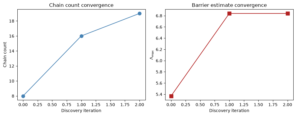
Automatic chain count discovery#
How many chains do we need? Too few and swaps are rejected too often; too many wastes computation. tune_chains iteratively probes different chain counts to find the right number.
The bootstrapping problem: \(\Lambda\) estimated with too few chains is biased low (the coarse schedule can't resolve the peak in \(\lambda(\beta)\)). The discovery algorithm handles this by iteratively refining.
def init_factory(n_chains, ebms_list, programs_list):
    """Create initial states for a given number of chains."""
    fb = programs_list[0].gibbs_spec.free_blocks
    ks = jax.random.split(jax.random.key(0), n_chains)
    return [hinton_init(ks[i], ebms_list[0], fb, ()) for i in range(n_chains)]


disc_key = jax.random.key(42)
discovery = tune_chains(
    disc_key,
    init_factory=init_factory,
    clamp_state=[],
    beta_range=(0.3, 1.0),
    gibbs_steps_per_round=GIBBS_STEPS,
    initial_n=8,
    target_acceptance=0.6,
    ebm=ebm,
    program=program,
)

print("=== Chain Count Discovery ===")
print(f"Final chain count: {discovery['n_chains']}")
print(f"Barrier estimate \u039b: {discovery['Lambda']:.4f}")
print(f"Convergence reason: {discovery['converged_reason']}")
print("\nDiscovery history:")
for entry in discovery["history"]:
    print(
        f"  Iter {entry['iteration']}: n={entry['n']}, \u039b_raw={entry['Lambda_raw']:.3f}, "
        f"\u039b_max={entry['Lambda_max']:.3f}, n_rec={entry['n_recommended']}"
    )
=== Chain Count Discovery ===
Final chain count: 19
Barrier estimate Λ: 6.8400
Convergence reason: chain_count

Discovery history:
  Iter 0: n=8, Λ_raw=5.370, Λ_max=5.370, n_rec=16
  Iter 1: n=16, Λ_raw=6.840, Λ_max=6.840, n_rec=19
  Iter 2: n=19, Λ_raw=6.660, Λ_max=6.840, n_rec=19
# Plot discovery convergence
hist = discovery["history"]
iters = [e["iteration"] for e in hist]
ns = [e["n"] for e in hist]
lambdas_disc = [e["Lambda_max"] for e in hist]

fig, axes = plt.subplots(1, 2, figsize=(10, 4))

axes[0].plot(iters, ns, "o-", color="steelblue", markersize=8)
axes[0].set_xlabel("Discovery iteration")
axes[0].set_ylabel("Chain count")
axes[0].set_title("Chain count convergence")

axes[1].plot(iters, lambdas_disc, "s-", color="firebrick", markersize=8)
axes[1].set_xlabel("Discovery iteration")
axes[1].set_ylabel("$\\Lambda_{\\max}$")
axes[1].set_title("Barrier estimate convergence")

plt.tight_layout()
plt.show()
Head-to-head: naive vs optimized vs more chains#
Everything above builds toward a single question: does this actually help? Let's run the same model with three configurations and compare:
- Naive: uniform \(\beta\) spacing, no schedule tuning, 8 chains
- Optimized: adaptive schedule, 16 chains
- Naive (16 chains): double the chains, still uniform spacing
The punchline: optimization with 16 chains should beat naive with 16.
# Fresh model so all three configs use identical graphs
L_cmp = 16
nodes_cmp, nodes_2d_cmp, edges_cmp, biases_cmp, weights_cmp, fb_cmp = make_ising_grid(
    L_cmp, coupling=1.0
)


def run_experiment(key, betas_arr, label):
    """Run NRPT and collect timing + diagnostics."""
    nc = len(betas_arr)
    ebm_list = [
        IsingEBM(nodes_cmp, edges_cmp, biases_cmp, weights_cmp, jnp.array(float(b)))
        for b in betas_arr
    ]
    prog_list = [IsingSamplingProgram(e, fb_cmp, []) for e in ebm_list]
    ks = jax.random.split(jax.random.key(0), nc + 1)
    inits = [hinton_init(ks[i], ebm_list[0], fb_cmp, ()) for i in range(nc)]

    # Warmup (compile)
    _ = nrpt(
        ks[-1], ebm_list, prog_list, inits, [], n_rounds=2, gibbs_steps_per_round=1
    )

    k_run = jax.random.key(
        {"Naive (8 chains)": 1, "Optimized (16 chains)": 2, "Naive (16 chains)": 3}[
            label
        ]
    )
    t0 = time.perf_counter()
    _, st = nrpt(
        k_run,
        ebm_list,
        prog_list,
        inits,
        [],
        n_rounds=N_ROUNDS,
        gibbs_steps_per_round=GIBBS_STEPS,
    )
    jax.block_until_ready(st["accepted"])
    elapsed = time.perf_counter() - t0

    d = st["round_trip_diagnostics"]
    return {
        "label": label,
        "n_chains": nc,
        "elapsed": elapsed,
        "Lambda": float(d["Lambda"]),
        "tau_predicted": float(d["tau_predicted"]),
        "tau_observed": float(d["tau_observed"]),
        "efficiency": float(d["efficiency"]),
        "total_round_trips": int(jnp.sum(d["round_trips_per_chain"])),
        "rejection_rates": np.array(st["rejection_rates"]),
        "betas": np.array(st["betas"]),
    }
# Template EBM and program for the comparison grid
cmp_ebm = IsingEBM(nodes_cmp, edges_cmp, biases_cmp, weights_cmp, jnp.array(1.0))
cmp_prog = IsingSamplingProgram(cmp_ebm, fb_cmp, [])

# A: Naive, 8 chains, uniform beta
result_naive = run_experiment(
    jax.random.key(42), jnp.linspace(0.3, 1.0, 8), "Naive (8 chains)"
)

# B: Optimized, 16 chains -- run adaptive on the comparison grid
key_opt16 = jax.random.key(42)
ks_opt = jax.random.split(key_opt16, 17)
# Build initial EBMs at uniform betas to get init states
init_betas_16 = jnp.linspace(0.3, 1.0, 16)
init_ebms_16 = [cmp_ebm.with_beta(jnp.array(float(b))) for b in init_betas_16]
inits_opt16 = [hinton_init(ks_opt[i], init_ebms_16[0], fb_cmp, ()) for i in range(16)]
_, stats_opt16 = tune_schedule(
    ks_opt[-1],
    init_states=inits_opt16,
    clamp_state=[],
    n_rounds=500,
    gibbs_steps_per_round=GIBBS_STEPS,
    initial_betas=init_betas_16,
    n_tune=4,
    rounds_per_tune=400,
    ebm=cmp_ebm,
    program=cmp_prog,
)
result_opt = run_experiment(
    jax.random.key(42), stats_opt16["betas"], "Optimized (16 chains)"
)

# C: Naive, 16 chains, uniform beta
result_more = run_experiment(
    jax.random.key(42), jnp.linspace(0.3, 1.0, 16), "Naive (16 chains)"
)

results = [result_naive, result_opt, result_more]
# Comparison table
col_w = 14
hdr = f"{'':32s} {'Naive 8':>{col_w}s} {'Opt 16':>{col_w}s} {'Naive 16':>{col_w}s}"
print(hdr)
print("-" * len(hdr))

fields = [
    ("Chains", "n_chains", "d"),
    ("Wall time (s)", "elapsed", ".2f"),
    ("Barrier \u039b", "Lambda", ".4f"),
    ("\u03c4 predicted", "tau_predicted", ".4f"),
    ("\u03c4 observed", "tau_observed", ".4f"),
    ("Efficiency (\u03c4/\u03c4\u0304)", "efficiency", ".2%"),
    ("Total round trips", "total_round_trips", "d"),
    ("Round trips / sec", None, ".1f"),
]

for label, key_name, fmt in fields:
    vals = []
    for r in results:
        if key_name is None:
            v = r["total_round_trips"] / max(r["elapsed"], 1e-9)
        else:
            v = r[key_name]
        vals.append(f"{v:{fmt}}")
    print(f"{label:32s} {vals[0]:>{col_w}s} {vals[1]:>{col_w}s} {vals[2]:>{col_w}s}")
Naive 8         Opt 16       Naive 16
-----------------------------------------------------------------------------
Chains                                        8             16             16
Wall time (s)                              0.38           0.60           0.28
Barrier Λ                                4.6200         6.5900         6.2040
τ predicted                              0.0890         0.0659         0.0694
τ observed                               0.0030         0.0270         0.0170
Efficiency (τ/τ̄)                         3.37%         40.99%         24.49%
Total round trips                             3             27             17
Round trips / sec                           7.8           44.9           61.0
Full pipeline: discover → adapt → sample#
Let's put it all together: use tune_chains to find the right number of chains, then tune_schedule to optimize the schedule and collect production samples from the cold chain.
# Collect samples using NRPT observer
n_production_rounds = 1000
n_opt = discovery["n_chains"]
init_betas = jnp.linspace(0.3, 1.0, n_opt)

key_pipe = jax.random.key(42)
k_tune, k_prod = jax.random.split(key_pipe)

# First: tune the schedule
init_ebms = [ebm.with_beta(jnp.array(float(b))) for b in init_betas]
init_progs = [program.with_ebm(e) for e in init_ebms]
init_opt = init_factory(n_opt, init_ebms, init_progs)

states_tuned, stats_tuned = tune_schedule(
    k_tune,
    init_states=init_opt,
    clamp_state=[],
    n_rounds=500,
    gibbs_steps_per_round=GIBBS_STEPS,
    initial_betas=init_betas,
    n_tune=4,
    rounds_per_tune=400,
    ebm=ebm,
    program=program,
)

# Production: single nrpt call with observer collects all cold-chain states
opt_betas = stats_tuned["betas"]
opt_ebms = [ebm.with_beta(jnp.array(float(b))) for b in opt_betas]
opt_progs = [program.with_ebm(e) for e in opt_ebms]

obs = NRPTStateObserver(chain_indices=(-1,))

_, stats_prod = nrpt(
    k_prod,
    opt_ebms,
    opt_progs,
    states_tuned,
    [],
    n_rounds=n_production_rounds,
    gibbs_steps_per_round=GIBBS_STEPS,
    betas=opt_betas,
    observer=obs,
)

# observations is a list of arrays, one per block, each (n_rounds, 1, ...)
# Squeeze out the chain dim and flatten across blocks
cold_per_block = [arr[:, 0] for arr in stats_prod["observations"]]
final_samples = jnp.concatenate(
    [c.reshape(n_production_rounds, -1) for c in cold_per_block], axis=1
)

rt_final = stats_prod["round_trip_diagnostics"]
print(f"Chains used: {n_opt}")

print(f"Round trips: {rt_final['round_trips_per_chain']}")
print(f"τ predicted: {float(rt_final['tau_predicted']):.4f}")
print(f"Rejection rates: {[f'{float(r):.3f}' for r in stats_prod['rejection_rates']]}")
print(f"Final samples: {final_samples.shape}")
print(f"Final Λ: {float(rt_final['Lambda']):.4f}")
print(f"Final efficiency: {float(rt_final['efficiency']):.4f}")
Chains used: 19
Round trips: [0 3 1 0 0 2 1 2 2 1 1 2 1 3 1 2 1 1 1]
τ predicted: 0.0662
Rejection rates: ['0.328', '0.366', '0.372', '0.364', '0.456', '0.432', '0.394', '0.346', '0.368', '0.374', '0.412', '0.368', '0.292', '0.378', '0.292', '0.330', '0.384', '0.302']
Final samples: (1000, 256)
Final Λ: 6.5580
Final efficiency: 0.3779
# Verify sample quality
from hamon.diagnostics import sample_convergence, marginal_entropy
report = sample_convergence(final_samples)
entropy = marginal_entropy(final_samples)
print(f"Convergence status: {report.status}")
print(f"Marginal entropy: {entropy:.4f}")
print()
print("Note: convergence reports 'NEED_MORE' and rank stability is meaningless here")
print(
"because this is a symmetric ferromagnet — all 256 spins have identical marginals."
)
print("The entropy of ~1.0 is the meaningful diagnostic: PT is sampling both modes.")
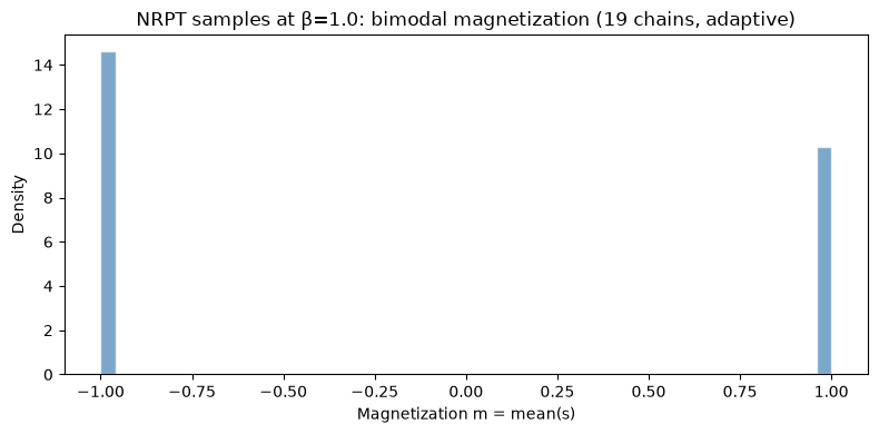
# Magnetization histogram
spins = 2.0 * final_samples.astype(float) - 1.0 # bool -> +/-1
mag = spins.mean(axis=1)
fig, ax = plt.subplots(figsize=(8, 4))
ax.hist(mag, bins=50, density=True, alpha=0.7, color="steelblue", edgecolor="white")
ax.set_xlabel("Magnetization m = mean(s)")
ax.set_ylabel("Density")
ax.set_title(f"NRPT samples at β=1.0: bimodal magnetization ({n_opt} chains, adaptive)")
plt.tight_layout()
plt.show()
Convergence status: NEED_MORE
Marginal entropy: 0.9787

Note: convergence reports 'NEED_MORE' and rank stability is meaningless here
because this is a symmetric ferromagnet — all 256 spins have identical marginals.
The entropy of ~1.0 is the meaningful diagnostic: PT is sampling both modes.
Summary#
- Parallel tempering overcomes energy barriers by running chains at multiple temperatures and swapping states
- DEO swaps (deterministic even-odd) provide non-reversibility, improving round trip rates over random swaps
- hamon exploits temperature linearity for efficient swap decisions (one energy eval per chain)
- Round trip diagnostics (\(\Lambda\), \(\tau\), efficiency) quantify sampling quality
- Adaptive schedule optimization concentrates chains near the phase transition bottleneck, reducing \(\Lambda\)
- Chain count discovery automatically finds the right number of chains
- The head-to-head comparison shows that optimized 16 chains beats naive 16 chains — smart scheduling matters more than raw chain count